AP Statistics Chapter 1

The average; most common measure of centrality; not resistant.

The midpoint; resistant; the same as the mean if the data set is symmetric. Example: [14, 21, 23, 23] Middle numbers are 21 and 23. 21 + 23 = 44
44 ÷ 2 = 22

Shows spread of the middle half of the data. Q₁(lower quartile): cuts off lowest 25% of data; 25th percentile; median of the lower half of the data. Q₃(upper quartile): cuts off lowest 75%; 75th percentile; median of the upper half of the data. Example: [3, 6, 7, 7, 8, 8, 9, 10, 12, 12, 15] Q₁=7 Q₃=12

The best measure for finding outliers; the middle 50% of a data set. Formula: Q₃-Q₁

A point that falls outside the IQR x 1.5 + maximum value, or the IQR x 1.5 - minimum value. Example of finding outliers: [3, 6, 7, 7, 8, 8, 9, 10, 12, 12, 15] (Q₃-Q₁): 12-7=5 (formula for finding outliers)1.5 x 5= 7.5 15(maximum)+7.5=22.5(upper outlier minimum) 3(minimum) - 7.5=-4.5(lower outlier maximum)

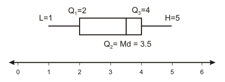
Has a data set's minimum value, lower quartile, median, upper quartile, maximum value; itself can create a boxplot.

A graph that uses the five number summary.

S²; the average of the squares of the deviations of values from the mean

Measures the spread by seeing how far the values are from the mean; the square root of the variance; not resistant; should only be used if the mean of a data set is chosen as its measure of centrality.

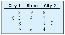
Good for comparing the shapes of 2 data sets or small numbers of quantitative values, but for comparing the centers or the spreads, a side-by-side boxplot would be better. They both are effective in comparing quantitative distributions. Example (with picture): City 1[32, 43, 48, 56, 69] City 2[38, 41, 51, 57, 64]